Tutorial 1 - Spatial analysis with Python

Attention

Finnish university students are encouraged to use the CSC Notebooks platform. If you haven’t used the CSC Notebooks before, see instructions to get started.

Others can follow the lesson interactively using Binder. Check the rocket icon on the top of this page.

In this tutorial, we will take a quick tour to Python’s (spatial) data science ecosystem and see how we can use some of the fundamental open source Python packages, such as:

• pandas / geopandas

• shapely

• pysal

• pyproj

• osmnx

• matplotlib (visualization)

As you can see, we won’t use any GIS software for doing the programming (such as ArcGIS/arcpy or QGIS), but focus on learning the open source packages that are independent from any specific software. These libraries form nowadays not only the core for modern spatial data science, but they are also fundamental parts of commercial applications used and developed by many companies around the world.

Note

If you have experience working with the Python’s spatial data science stack, this tutorial probably does not bring much new to you, but to get everyone on the same page, we will all go through this introductory tutorial.

Contents

• Reading / writing spatial data

• Retrieving OpenStreetMap data

• Reprojections

• Spatial join

• Plotting data with matplotlib

Getting started

There are two options for running the codes in this tutorial:

1. Run the codes using CSC Notebooks (see the top of this page) which is the easiest way and recommended if you do not have experience installing Python software. With this option you have slightly limited computational resources (10 GB memory).

2. Download this Notebook (see instructions below) and run it using Jupyter Lab which you should have installed by following the installation instructions.

Run the tutorial using own computer (optional - requires installations)

See the instructions

Download the Notebook

You can download this tutorial Notebook to your own computer by clicking the Download button from the Menu on the top-right section of the website.

• Right-click the option that says .ipynb and choose “Save link as ..”

Run the codes on your own computer

Before you can run this Notebook, and/or do any programming, you need to launch the Jupyter Lab programming environment. The JupyterLab comes with the environment that you installed earlier (if you have not done this yet, follow the installation instructions). To run the JupyterLab:

1. Using terminal/command prompt, navigate to the folder where you have downloaded the Jupyter Notebook tutorial: $ cd /mydirectory/

2. Activate the programming environment: $ conda activate geo

3. Launch the JupyterLab: $ jupyter lab

After these steps, the JupyterLab interface should open, and you can start executing cells (see hints below at “Working with Jupyter Notebooks”).

Download the data

If you use your own computer, DOWNLOAD THE DATA to your own computer and extract it to the same location where you have downloaded this notebook. Inside the ZIP file, there is a folder called data which is used in the following parts of the tutorial.

Working with Jupyter Notebooks

Jupyter Notebooks are documents that can be used and run inside the JupyterLab programming environment containing the computer code and rich text elements (such as text, figures, tables and links).

A couple of hints:

• You can execute a cell by clicking a given cell that you want to run and pressing Shift + Enter (or by clicking the “Play” button on top)

• You can change the cell-type between Markdown (for writing text) and Code (for writing/executing code) from the dropdown menu above.

See further details and help for using Notebooks and JupyterLab from here.

Fundamental library: Geopandas

In this course, the most often used Python package that you will learn is geopandas. Geopandas makes it possible to work with geospatial data in Python in a relatively easy way. Geopandas combines the capabilities of the data analysis library pandas with other packages like shapely and fiona for managing spatial data. The main data structures in geopandas are GeoSeries and GeoDataFrame which extend the capabilities of Series and DataFrames from pandas. In case you wish to have additional help getting started with pandas, we recommend you to take a look at Chapter 3 from the openly available Introduction to Python for Geographic Data Analysis -book. The main difference between GeoDataFrames and pandas DataFrames is that a GeoDataFrame should contain (at least) one column for geometries. By default, the name of this column is 'geometry'. The geometry column is a GeoSeries which contains the geometries (points, lines, polygons, multipolygons etc.) as shapely objects.

Reading and writing spatial data

Next we will learn some of the basic functionalities of geopandas. We have a couple of GeoJSON files stored in the data folder that we will use.

We can read the data easily with read_file() -function:

import geopandas as gpd

# Filepath
fp = "data/buildings.geojson"

# Read the file
data = gpd.read_file(fp)

# How does it look?
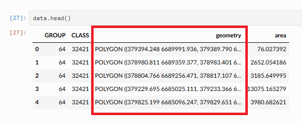
data.head()

	addr:city	addr:country	addr:housenumber	addr:housename	addr:postcode	addr:street	email	name	opening_hours	operator	...	start_date	wikipedia	id	timestamp	version	tags	osm_type	internet_access	changeset	geometry
0	Helsinki	NaN	29	NaN	00170	Unioninkatu	NaN	NaN	NaN	NaN	...	NaN	NaN	4253124	1542041335	4	NaN	way	NaN	NaN	POLYGON ((24.95121 60.16999, 24.95122 60.16988...
1	Helsinki	NaN	2	NaN	00100	Kaivokatu	ainfo@ateneum.fi	Ateneum	Tu, Fr 10:00-18:00; We-Th 10:00-20:00; Sa-Su 1...	NaN	...	1887	fi:Ateneumin taidemuseo	8033120	1544822447	27	{'architect': 'Theodor Höijer', 'contact:websi...	way	NaN	NaN	POLYGON ((24.94477 60.16982, 24.94450 60.16981...
2	Helsinki	FI	22-24	NaN	NaN	Mannerheimintie	NaN	Lasipalatsi	NaN	NaN	...	1936	fi:Lasipalatsi	8035238	1533831167	23	{'name:fi': 'Lasipalatsi', 'name:sv': 'Glaspal...	way	NaN	NaN	POLYGON ((24.93561 60.17045, 24.93555 60.17054...
3	Helsinki	NaN	2	NaN	00100	Mannerheiminaukio	NaN	Kiasma	Tu 10:00-17:00; We-Fr 10:00-20:30; Sa 10:00-18...	NaN	...	1998	fi:Kiasma (rakennus)	8042215	1553963033	30	{'name:en': 'Museum of Modern Art Kiasma', 'na...	way	NaN	NaN	POLYGON ((24.93682 60.17152, 24.93662 60.17150...
4	NaN	FI	NaN	NaN	NaN	NaN	NaN	NaN	NaN	NaN	...	NaN	NaN	15243643	1546289715	7	NaN	way	NaN	NaN	POLYGON ((24.93675 60.16779, 24.93660 60.16789...

5 rows × 34 columns

As we can see, the GeoDataFrame contains various attributes in separate columns. The geometry column contains the spatial information. We can take a look of some of the basic information about our GeoDataFrame with command:

data.info()

<class 'geopandas.geodataframe.GeoDataFrame'>
RangeIndex: 486 entries, 0 to 485
Data columns (total 34 columns):
 #   Column              Non-Null Count  Dtype   
---  ------              --------------  -----   
 0   addr:city           86 non-null     object  
 1   addr:country        57 non-null     object  
 2   addr:housenumber    88 non-null     object  
 3   addr:housename      4 non-null      object  
 4   addr:postcode       54 non-null     object  
 5   addr:street         89 non-null     object  
 6   email               2 non-null      object  
 7   name                81 non-null     object  
 8   opening_hours       8 non-null      object  
 9   operator            7 non-null      object  
 10  phone               8 non-null      object  
 11  ref                 1 non-null      object  
 12  url                 8 non-null      object  
 13  website             20 non-null     object  
 14  building            486 non-null    object  
 15  amenity             26 non-null     object  
 16  building:levels     162 non-null    object  
 17  building:material   2 non-null      object  
 18  building:min_level  4 non-null      object  
 19  height              17 non-null     object  
 20  landuse             2 non-null      object  
 21  office              5 non-null      object  
 22  shop                5 non-null      object  
 23  source              3 non-null      object  
 24  start_date          87 non-null     object  
 25  wikipedia           47 non-null     object  
 26  id                  486 non-null    int64   
 27  timestamp           486 non-null    int64   
 28  version             486 non-null    int64   
 29  tags                181 non-null    object  
 30  osm_type            486 non-null    object  
 31  internet_access     1 non-null      object  
 32  changeset           66 non-null     float64 
 33  geometry            486 non-null    geometry
dtypes: float64(1), geometry(1), int64(3), object(29)
memory usage: 129.2+ KB

From here, we can see that our data is indeed a GeoDataFrame object with 486 entries and 34 columns. You can also get descriptive statistics of your data by calling:

data.describe()

	id	timestamp	version	changeset
count	4.860000e+02	4.860000e+02	486.000000	66.0
mean	1.400780e+08	1.455829e+09	4.849794	0.0
std	1.633527e+08	9.247528e+07	4.561162	0.0
min	8.253000e+03	1.197929e+09	1.000000	0.0
25%	2.294267e+07	1.374229e+09	2.000000	0.0
50%	1.228699e+08	1.493288e+09	3.000000	0.0
75%	1.359805e+08	1.530222e+09	7.000000	0.0
max	1.042029e+09	1.555840e+09	31.000000	0.0

In this case, we didn’t have many columns with numerical data, but typically you have numeric values in your dataset and this is a good way to get a quick view how the data look like.

Naturally, as the data is spatial, we want to visualize it to understand the nature of the data better. We can do this easily with plot() method:

data.plot()

<Axes: >

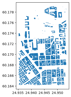
Now we can see that the data indeed represents buildings (in central Helsinki). Naturally we can also write this data to disk. Geopandas supports writing data to various data formats as well as to PostGIS which is the most widely used open source database for GIS. Let’s write the data as a Shapefile to the same data directory from where we read the data. When writing data to local disk you can use to_file() method that exports the data in Shapefile format by default:

# Output filepath
outfp = "data/buildings_copy.shp"
data.to_file(outfp)

/tmp/ipykernel_350523/403506898.py:3: UserWarning: Column names longer than 10 characters will be truncated when saved to ESRI Shapefile.
  data.to_file(outfp)

Retrieving data from OpenStreetMap

Now we have seen how to read spatial data from disk. OpenStreetMap (OSM) is probably the most well known and widely used spatial dataset/database in the world. Also in this course, we will use OSM data frequently. Hence, let’s see how we can retrieve data from OSM using a library called omsnx. With osmnx you can easily download and extract data from anywhere in the world based on the Overpass API. You can use osmnx e.g. to retrieve OSM data around a given address and applying a 2 km buffer around this location. Hence, osmnx is a very flexible library in terms of specifying the area of interest.

OSM is a “database of the world”, hence it contains a lot of information about different things. With osmnx you can easily extract information about:

• street networks –> ox.graph_from_place(query) | ox.graph_from_polygon(polygon)

• buildings –> ox.features_from_place(query, tags={"buildings": True}) | ox.features_from_polygon(polygon, tags={"buildings": True})

• Amenities –> ox.features_from_place(query, tags={"amenity": True}) | ox.features_from_polygon(polygon, tags={"amenity": True})

• landuse –> ox.features_from_place(query, tags={"landuse": True}) | ox.features_from_polygon(polygon, tags={"landuse": True})

• natural elements –> ox.features_from_place(query, tags={"natural": True}) | ox.features_from_polygon(polygon, tags={"natural": True})

• boundaries –> ox.features_from_place(query, tags={"boundary": True}) | ox.features_from_polygon(polygon, tags={"boundary": True})

Let’s see how we can download and extract OSM data about buildings for Helsinki central area using osmnx:

import osmnx as ox
from shapely.geometry import box

# Bounding box for given area (Helsinki city centre)
bounds = [24.9351773, 60.1641551, 24.9534055, 60.1791068]

# Create a bounding box Polygon
bbox = box(*bounds)

# Retrieve buildings from the given area
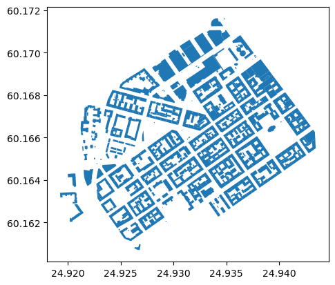
buildings = ox.features_from_polygon(bbox, tags={"building": True})

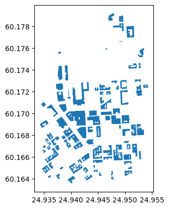
buildings.plot()

<Axes: >

buildings.head()

		geometry	addr:city	addr:country	addr:housenumber	addr:postcode	addr:street	air_conditioning	brand	building	contact:facebook	...	name:ja	opening_hours:covid19	payment:cash	payment:mastercard	name:cs	ways	type	last_roof_renovation	electrified	nohousenumber
element_type	osmid
node	55211772	POINT (24.95158 60.17716)	Helsinki	FI	4	00530	John Stenbergin ranta	yes	Hilton Hotels & Resorts	yes	https://www.facebook.com/HiltonHelsinkiStrand/	...	NaN	NaN	NaN	NaN	NaN	NaN	NaN	NaN	NaN	NaN
	5643347516	POINT (24.94393 60.17412)	NaN	NaN	NaN	NaN	NaN	NaN	NaN	roof	NaN	...	NaN	NaN	NaN	NaN	NaN	NaN	NaN	NaN	NaN	NaN
way	4253124	POLYGON ((24.95121 60.16999, 24.95122 60.16987...	Helsinki	NaN	29	00170	Unioninkatu	NaN	NaN	religious	NaN	...	NaN	NaN	NaN	NaN	NaN	NaN	NaN	NaN	NaN	NaN
	8033120	POLYGON ((24.94477 60.16982, 24.94450 60.16981...	Helsinki	NaN	2	00100	Kaivokatu	NaN	NaN	museum	NaN	...	NaN	NaN	NaN	NaN	NaN	NaN	NaN	NaN	NaN	NaN
	8035238	POLYGON ((24.93563 60.17045, 24.93557 60.17054...	Helsinki	FI	22-24	NaN	Mannerheimintie	NaN	NaN	public	NaN	...	NaN	NaN	NaN	NaN	NaN	NaN	NaN	NaN	NaN	NaN

5 rows × 150 columns

Let’s check how many buildings did we get:

len(buildings)

545

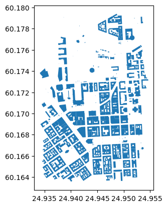
Okay, so in this sample there are over 500 buildings in the Helsinki city center area. Naturally, we would like to see them on a map. Let’s plot our data using plot() (might take some time as there are many objects to plot):

buildings.plot()

<Axes: >

Great! As a result we got a map that seems to look correct.

Reprojecting data

As we can see from the previous maps that we have produced, the coordinates on the x and y axis hint that our geometries are represented in decimal degrees (WGS84). In many cases, you want to reproject your data to another CRS. Luckily, doing that is easy with geopandas. Let’s first take a look what the Coordinate Reference System (CRS) of our GeoDataFrame is. We can access the CRS information of the GeoDataFrame by accessing an attribute called crs:

buildings.crs

<Geographic 2D CRS: EPSG:4326>
Name: WGS 84
Axis Info [ellipsoidal]:
- Lat[north]: Geodetic latitude (degree)
- Lon[east]: Geodetic longitude (degree)
Area of Use:
- name: World.
- bounds: (-180.0, -90.0, 180.0, 90.0)
Datum: World Geodetic System 1984 ensemble
- Ellipsoid: WGS 84
- Prime Meridian: Greenwich

As a result, we get information about the CRS, and we can see that the data is indeed in WGS84. We can also see that the EPSG code for the CRS is 4326. We can easily reproject our data by using a method to_crs(). The easiest way to use the method is to specify the destination CRS as an EPSG code. Let’s reproject our data into EPSG 3067 which is the most widely used projected coordinate reference system used in Finland, EUREF-FIN:

projected = buildings.to_crs(epsg=3067)
projected.crs

<Projected CRS: EPSG:3067>
Name: ETRS89 / TM35FIN(E,N)
Axis Info [cartesian]:
- E[east]: Easting (metre)
- N[north]: Northing (metre)
Area of Use:
- name: Finland - onshore and offshore.
- bounds: (19.08, 58.84, 31.59, 70.09)
Coordinate Operation:
- name: TM35FIN
- method: Transverse Mercator
Datum: European Terrestrial Reference System 1989 ensemble
- Ellipsoid: GRS 1980
- Prime Meridian: Greenwich

As we can see, now we have an Projected CRS as a result. To confirm the difference, let’s take a look at the geometry of the first row in our original buildings GeoDataFrame and the projected GeoDataFrame. To select a specific row in data, we can use the iloc indexing:

orig_geom = buildings.iloc[3]["geometry"]
projected_geom = projected.iloc[3]["geometry"]

print("Orig:\n", orig_geom, "\n")
print("Proj:\n", projected_geom)

Orig:
 POLYGON ((24.9447717 60.1698154, 24.9444956 60.1698084, 24.9444744 60.1698084, 24.9444736 60.169802, 24.9444699 60.1697974, 24.944464 60.1697933, 24.9444515 60.1697904, 24.9444407 60.1697895, 24.9444291 60.1697902, 24.9444176 60.169794, 24.9444099 60.1697989, 24.9444077 60.1698096, 24.9443866 60.1698091, 24.9442857 60.1698068, 24.9442881 60.1698043, 24.9441174 60.1697997, 24.9439045 60.1697951, 24.9438447 60.1697943, 24.9437851 60.1697936, 24.9437838 60.1697863, 24.9437774 60.1697816, 24.943767 60.1697764, 24.9437553 60.1697744, 24.9437415 60.1697761, 24.9437291 60.1697792, 24.9437204 60.1697846, 24.943718 60.1697918, 24.9436953 60.1697923, 24.9436953 60.1697854, 24.9434197 60.1697794, 24.9434198 60.1697827, 24.9434107 60.1697825, 24.9434073 60.1698027, 24.9434038 60.1698228, 24.9433519 60.1702316, 24.9433862 60.1702322, 24.9434032 60.1702326, 24.9434032 60.1702243, 24.9434407 60.1702246, 24.9434414 60.1702333, 24.9434997 60.1702353, 24.9435004 60.1702286, 24.9438646 60.1702385, 24.9438639 60.1702556, 24.9439289 60.1702557, 24.9439293 60.1702649, 24.9439752 60.1702654, 24.9439762 60.170256, 24.9439831 60.1702563, 24.9440485 60.1702588, 24.9441197 60.1702607, 24.94412 60.1702694, 24.944163 60.1702705, 24.9441635 60.1702623, 24.9442303 60.1702633, 24.9442314 60.1702489, 24.9445891 60.1702567, 24.9445884 60.1702644, 24.9446412 60.1702642, 24.9446421 60.1702583, 24.9446796 60.1702595, 24.944679 60.1702648, 24.9447086 60.1702648, 24.9447401 60.1702653, 24.9447441 60.1702197, 24.9447539 60.1702199, 24.9447589 60.1701626, 24.9447625 60.1701626, 24.9447637 60.1701487, 24.9447508 60.1701484, 24.9447538 60.1701141, 24.9447574 60.1701142, 24.9447585 60.1701021, 24.9447491 60.1701019, 24.9447638 60.1699327, 24.9447764 60.169933, 24.9447782 60.1699128, 24.9447742 60.1699128, 24.9447772 60.1698775, 24.9447819 60.1698776, 24.9447837 60.1698571, 24.9447794 60.169857, 24.9447813 60.1698368, 24.9447829 60.1698156, 24.9447717 60.1698154)) 

Proj:
 POLYGON ((385964.4830272406 6672097.9406245435, 385949.1425152434 6672097.638128187, 385947.96647580387 6672097.674744761, 385947.8999115388 6672096.963586301, 385947.6787135364 6672096.457838686, 385947.33720683504 6672096.01155816, 385946.63373416744 6672095.710278626, 385946.03149954154 6672095.628731746, 385945.39043248596 6672095.726701813, 385944.76565917226 6672096.169635931, 385944.3554988305 6672096.728474411, 385944.27054940484 6672097.92355255, 385943.09832408716 6672097.904330759, 385937.49306880624 6672097.822548425, 385937.6175383835 6672097.540066742, 385928.13225308526 6672097.32280155, 385916.3059809507 6672097.178468479, 385912.98588742805 6672097.192718051, 385909.6772352841 6672097.217758516, 385909.5798059091 6672096.407263622, 385909.2084770431 6672095.895049865, 385908.6135198497 6672095.334080153, 385907.95754336845 6672095.131626718, 385907.19790274795 6672095.344739051, 385906.5207800623 6672095.711300708, 385906.05688559415 6672096.327538558, 385905.94871675764 6672097.1332929395, 385904.69120054704 6672097.228182361, 385904.66727283853 6672096.459975124, 385889.3579444295 6672096.268199428, 385889.37493700767 6672096.635430047, 385888.8694337494 6672096.628888855, 385888.75088261557 6672098.883718724, 385888.62643754866 6672101.12758798, 385887.1652323891 6672146.730769827, 385889.0700312803 6672146.738295941, 385890.014456613 6672146.75345202, 385889.98566978925 6672145.829376676, 385892.0669416933 6672145.797974151, 385892.13594626007 6672146.765373616, 385895.3769481551 6672146.887297964, 385895.39254267106 6672146.140147998, 385915.6300777834 6672146.61307313, 385915.65054132417 6672148.518100683, 385919.2566196625 6672148.416935189, 385919.3107089129 6672149.440520588, 385921.85864313797 6672149.416889636, 385921.88152304647 6672148.368618673, 385922.26532552345 6672148.390098511, 385925.90191431006 6672148.5554510765, 385929.8581645404 6672148.643987164, 385929.9049700098 6672149.612078236, 385932.2941130407 6672149.660264898, 385932.29341993807 6672148.746459043, 385936.0024690606 6672148.742401588, 385936.01356582344 6672147.137285974, 385955.88322852115 6672147.387859188, 385955.8710880219 6672148.246343194, 385958.7993581761 6672148.132886917, 385958.8288330893 6672147.4744594805, 385960.91322255775 6672147.543297039, 385960.8983094256 6672148.134405698, 385962.54030407744 6672148.083286338, 385964.28943007067 6672148.084553688, 385964.35327023955 6672143.000795997, 385964.8975975617 6672143.006138669, 385964.97635988146 6672136.618041293, 385965.1760625585 6672136.611824261, 385965.19445279264 6672135.062203406, 385964.4778114268 6672135.051080812, 385964.5253462377 6672131.2271291595, 385964.72539580934 6672131.232045548, 385964.74447754095 6672129.88299936, 385964.2223375002 6672129.876965906, 385964.45134616806 6672111.013795151, 385965.15135021566 6672111.025435871, 385965.1811898203 6672108.77337203, 385964.9592962705 6672108.7802798245, 385965.0033679507 6672104.844993874, 385965.2644397472 6672104.848010666, 385965.2932399619 6672102.562546515, 385965.05435739574 6672102.558838941, 385965.08974473877 6672100.306602424, 385965.10502421076 6672097.943549578, 385964.4830272406 6672097.9406245435))

As we can see the coordinates that form our Polygon has changed from decimal degrees to meters. Let’s see what happens if we just call the geometries:

orig_geom

projected_geom

As you can see, we can draw the geometry directly in the screen, and we can easily see the difference in the shape of the two geometries. The orig_geom and projected_geom variables contain a Shapely geometry which is Polygon in this case. We can confirm this by checking the type:

type(orig_geom)

shapely.geometry.polygon.Polygon

These shapely geometries are used as the underlying data structure in most GIS packages in Python to present geometrical information. Shapely is fundamentally a Python wrapper for GEOS which is widely used library (written in C++) under the hood of many GIS softwares such as QGIS, GDAL, GRASS, PostGIS, Google Earth etc. Currently, there is ongoing work to vectorize all the GEOS functionalities for Python and bring those eventually into Shapely which will greatly boost the performance of all geometry related operations in Python ecosystem (approaching the same efficiency as PostGIS). Some of these improvements can already be found under the hood of latest version of geopandas.

Calculating area

One thing that is quite often interesting to know when working with spatial data, is the area of the geometries. In geopandas, we can easily calculate e.g. the area for each of our buildings by:

projected["building_area"] = projected.area
projected["building_area"].describe()

count     545.000000
mean     1036.089874
std      1128.288787
min         0.000000
25%       237.165839
50%       773.503344
75%      1396.511916
max      8419.604239
Name: building_area, dtype: float64

We calculated the area by calling area which is the attribute containing information about areas of the buildings measured based on the map units of the data. Hence, in this case because our data is projected in Euref-FIN the units that we stored in "building_area" column are square meters. It’s important to always keep in mind the CRS when calculating areas, distances etc. with geometries.

Spatial join

A commonly needed GIS functionality, is to be able to merge information between two layers using location as the key. Hence, it is somewhat similar approach as table join but because the operation is based on geometries, it is called spatial join. Next, we will see how we can conduct a spatial join and merge information between two layers. We will read all restaurants from the OSM for Helsinki Region, and combine information from restaurants to the underlying building (restaurants typically are within buildings). We will again use osmnx for reading the data, but this time we will get all amenities with tags “restaurant”, “bar” or “pub”:

# Read restaurants
query = "Helsinki, Finland"
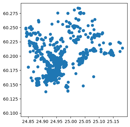
restaurants = ox.features_from_place(query, tags={"amenity": ["restaurant", "bar", "pub"]})
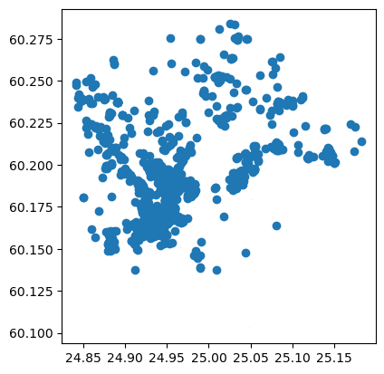
restaurants.plot()

<Axes: >

restaurants.info()

<class 'geopandas.geodataframe.GeoDataFrame'>
MultiIndex: 1598 entries, ('node', 25101780) to ('way', 1093942712)
Columns: 234 entries, addr:city to indoor
dtypes: geometry(1), object(233)
memory usage: 2.9+ MB

As we can see, the OSM for Helsinki contains more than 1500 restaurants altogether. As you can probably guess, the OSM data is far from “perfect” in terms of the quality of the restaurant listings. This is due to the voluntary nature of adding information to the OpenStreetMap, and the fact restaurants (as well as other POI features) are highly dynamic by nature, i.e. new amenities open and close all the time, and it is challenging to keep up to date with those changes (this is a challenge even for commercial companies).

Let’s also fetch buildings and administrative areas for the whole Helsinki area:

# Read buildings
query = "Helsinki, Finland"
hki_buildings = ox.features_from_place(query, tags={"building": True})

hki_buildings.plot()

<Axes: >

# Print the number of rows and columns
print(hki_buildings.shape)

# Show the first lines 
hki_buildings.head(2)

(63136, 674)

		geometry	amenity	check_date	operator	communication:mobile_phone	telecom	addr:city	addr:country	addr:housenumber	addr:postcode	...	architect:wikipedia	museum_type	blood:platelets	blood:whole	building:maintenance:operator:official_name	old_name:en	payment:american_express	payment:cheque	payment:diners_club	payment:maestro
element_type	osmid
node	55211772	POINT (24.95158 60.17716)	NaN	NaN	Hilton	NaN	NaN	Helsinki	FI	4	00530	...	NaN	NaN	NaN	NaN	NaN	NaN	NaN	NaN	NaN	NaN
	247474256	POINT (25.05441 60.20797)	car_wash	NaN	Autopesu-Center	NaN	NaN	NaN	NaN	NaN	NaN	...	NaN	NaN	NaN	NaN	NaN	NaN	NaN	NaN	NaN	NaN

2 rows × 674 columns

As we can see, the OSM data contains more than 60 thousand building features that are represented with a mix of different types of geometries, namely Polygons and Points which are visible with large blue points on the map. In our case, we are only interested in the footprints of the buildings because we want to make a spatial join between restaurants and buildings. Hence, we want to remove the Point objects from our data. Luckily, this is easy because the points are represented with a specific OSM element_type: “node”. We can see all OSM elements that are present in our data by checking the index levels:

# What kind of elements do we have?
hki_buildings.index.levels[0]

Index(['node', 'relation', 'way'], dtype='object', name='element_type')

From these, we are only interested in “way” and “relation” OSM elements which contain the building polygons. Hence, let’s select those:

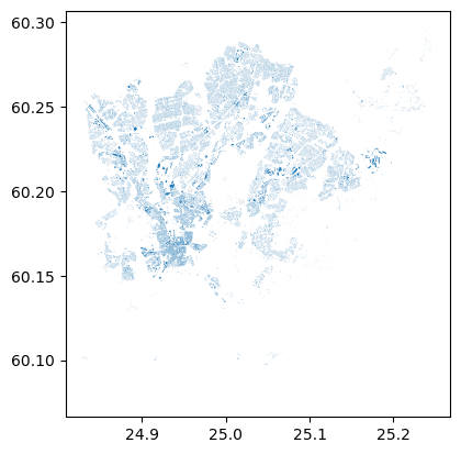
hki_buildings = hki_buildings.loc[(["way", "relation"])].copy()
hki_buildings.plot()

<Axes: >

Joining data from buildings to the restaurants can be done easily using sjoin() function from geopandas:

# Join information from buildings to restaurants
join = gpd.sjoin(restaurants, hki_buildings)

# Print column names
print(join.columns)

# Show rows
join

Index(['addr:city_left', 'addr:country_left', 'amenity_left', 'name_left',
       'geometry', 'contact:website_left', 'cuisine_left',
       'opening_hours_left', 'name:fi_left', 'name:sv_left',
       ...
       'architect:wikipedia', 'museum_type', 'blood:platelets', 'blood:whole',
       'building:maintenance:operator:official_name', 'old_name:en',
       'payment:american_express_right', 'payment:cheque',
       'payment:diners_club_right', 'payment:maestro'],
      dtype='object', length=909)

		addr:city_left	addr:country_left	amenity_left	name_left	geometry	contact:website_left	cuisine_left	opening_hours_left	name:fi_left	name:sv_left	...	architect:wikipedia	museum_type	blood:platelets	blood:whole	building:maintenance:operator:official_name	old_name:en	payment:american_express_right	payment:cheque	payment:diners_club_right	payment:maestro
element_type	osmid
node	25101780	Helsinki	FI	pub	Muusan Krouvi	POINT (24.85593 60.20729)	NaN	NaN	NaN	NaN	NaN	...	NaN	NaN	NaN	NaN	NaN	NaN	NaN	NaN	NaN	NaN
	25279508	NaN	NaN	restaurant	Pikku Ranska	POINT (24.86684 60.20897)	http://www.pikkuranska.com/	french	Mo-Th 10:30-22:15; Fr 11:00-23:00; Sa 12:00-23:00	NaN	NaN	...	NaN	NaN	NaN	NaN	NaN	NaN	NaN	NaN	NaN	NaN
	27392509	NaN	NaN	restaurant	Ravintola Seurasaari	POINT (24.88337 60.18118)	NaN	NaN	NaN	NaN	NaN	...	NaN	NaN	NaN	NaN	NaN	NaN	NaN	NaN	NaN	NaN
	50808688	NaN	NaN	pub	Foxy Bear	POINT (25.03395 60.20450)	NaN	NaN	Mo-Th 10:00-22:00; Fr 10:00-23:00; Sa 11:00-23...	NaN	NaN	...	NaN	NaN	NaN	NaN	NaN	NaN	NaN	NaN	NaN	NaN
	50808951	NaN	NaN	restaurant	Pikku-Hukka	POINT (25.03481 60.20454)	NaN	scandinavian	Tu 11:00-15:00; We 11:00-20:00; Th,Fr 11:00-21...	NaN	NaN	...	NaN	NaN	NaN	NaN	NaN	NaN	NaN	NaN	NaN	NaN
...	...	...	...	...	...	...	...	...	...	...	...	...	...	...	...	...	...	...	...	...	...	...
way	1079281914	Helsinki	NaN	bar	3-0 Sports Bar	POLYGON ((25.05189 60.17934, 25.05166 60.17932...	NaN	NaN	Mo-Sa 11:00-24:00; Su,PH 11:00-22:00	NaN	NaN	...	NaN	NaN	NaN	NaN	NaN	NaN	NaN	NaN	NaN	NaN
	1079281935	Helsinki	NaN	restaurant	GlassRoom	POLYGON ((25.05177 60.17933, 25.05189 60.17934...	NaN	NaN	NaN	NaN	NaN	...	NaN	NaN	NaN	NaN	NaN	NaN	NaN	NaN	NaN	NaN
	1079281940	Helsinki	NaN	restaurant	King Kebab	POLYGON ((25.05153 60.17989, 25.05158 60.17980...	NaN	kebab	Mo-Sa 10:30-22:00; Su,PH 11:30-21:00	NaN	NaN	...	NaN	NaN	NaN	NaN	NaN	NaN	NaN	NaN	NaN	NaN
	1079281941	Helsinki	NaN	restaurant	Fafa's	POLYGON ((25.05145 60.17971, 25.05161 60.17973...	NaN	middle_eastern	Mo-Sa 10:30-22:00; PH,Su 12:00-20:00	NaN	NaN	...	NaN	NaN	NaN	NaN	NaN	NaN	NaN	NaN	NaN	NaN
	1093942712	NaN	NaN	restaurant	NaN	POLYGON ((24.96990 60.19026, 24.96992 60.19026...	NaN	NaN	NaN	NaN	NaN	...	NaN	NaN	NaN	NaN	NaN	NaN	NaN	NaN	NaN	NaN

1606 rows × 909 columns

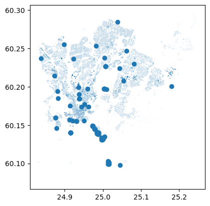
# Visualize the data as well
join.plot()

<Axes: >

As we can see from the above, now we have merged information from the buildings to restaurants. The geometries of the left GeoDataFrame, i.e. restaurants were kept by default as the geometries.

Select data based on spatial relationships

One handy trick and efficient trick for spatial join is to use it for selecting data. We can e.g. select all buildings that intersect with restaurants by conducting the spatial join other way around, i.e. using the buildings as the left GeoDataFrame and the restaurants as the right GeoDataFrame:

# Merge information from restaurants to buildings (conducts selection at the same time)
join2 = gpd.sjoin(buildings, restaurants, how="inner", predicate="intersects")
join2.plot()

<Axes: >

As we can see (although the small building geometries are a bit poorly visible), the end result is a layer of buildings which intersected with the restaurants. This is a straightforward way to conduct simple spatial queries. You can specify with predicate parameter whether the binary predicate between the layers (i.e. the spatial relation between geometries) should be:

• intersects

• contains

• within

Example: Select buildings for specific administrative area

In a similar manner, we can for example identify all buildings that are within a specific administrative area of Helsinki, such as Kamppi. Because OSM includes various different kinds of administrative boundaries (e.g. boundaries for the whole city vs postal code areas), we need to tell the osmnx to fetch only postal code areas. We can do this by using the OSM admin_level key. In Finland, the admin_level 10 stands for postal code areas, hence we fetch only those features from OSM:

# Fetch all admin borders for Helsinki
hki_admins = ox.features_from_place(query, tags={"admin_level": "10"})
hki_admins.plot()

<Axes: >

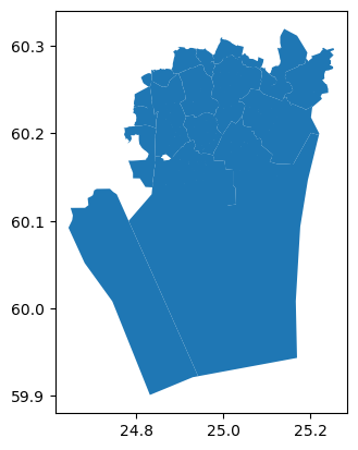
The name column in the OSM contains the names of all available postal code areas:

# Check all available districts based on values in "name" column
hki_admins.name.unique()

array([nan, 'Lauttasaari', 'Länsisatama', 'Eira', 'Ullanlinna',
       'Punavuori', 'Kaartinkaupunki', 'Katajanokka', 'Kruununhaka',
       'Kluuvi', 'Kamppi', 'Etu-Töölö', 'Taka-Töölö', 'Meilahti',
       'Laakso', 'Munkkiniemi', 'Kaivopuisto', 'Kallio', 'Sörnäinen',
       'Mustikkamaa-Korkeasaari', 'Alppiharju', 'Pasila', 'Vallila',
       'Hermanni', 'Ruskeasuo', 'Suomenlinna', 'Haaga', 'Pitäjänmäki',
       'Käpylä', 'Koskela', 'Kumpula', 'Toukola', 'Vanhakaupunki',
       'Oulunkylä', 'Kulosaari', 'Herttoniemi', 'Tammisalo', 'Laajasalo',
       'Villinki', 'Santahamina', 'Vartiosaari', 'Viikki', 'Konala',
       'Kaarela', 'Pakila', 'Tuomarinkylä', 'Pukinmäki', 'Malmi',
       'Ulkosaaret', 'Tapaninkylä', 'Suutarila', 'Suurmetsä',
       'Mellunkylä', 'Vartiokylä', 'Myyrmäki', 'Vapaala', 'Kaivoksela',
       'Vuosaari', 'Lintuvaara', 'Leppävaara', 'Ylästö', 'Pakkala',
       'Tammisto', 'Tikkurila', 'Talosaari', 'Salmenkallio',
       'Östersundom', 'Karhusaari', 'Ultuna', 'Sotunki',
       'Helsingin pitäjän kirkonkylä', 'Koivuhaka', 'Viertola',
       'Kuninkaala', 'Laajalahti', 'Otaniemi', 'Westend', 'Suvisaaristo',
       'Ojanko', 'Vaarala', 'Rajakylä', 'Länsisalmi', 'Länsimäki'],
      dtype=object)

We can now easily select only the data for Kamppi in Helsinki as follows:

# Select the boundaries for Kamppi
kamppi_admins = hki_admins.loc[hki_admins["name"] == "Kamppi"]

# Draw an interactive map
kamppi_admins.explore()

Make this Notebook Trusted to load map: File -> Trust Notebook

Finally, we can select all the buildings that belong to Kamppi:

# Select buildings within this area
kamppi_buildings = gpd.sjoin(hki_buildings, kamppi_admins, predicate="intersects")
kamppi_buildings.plot()

<Axes: >

Plotting data with matplotlib

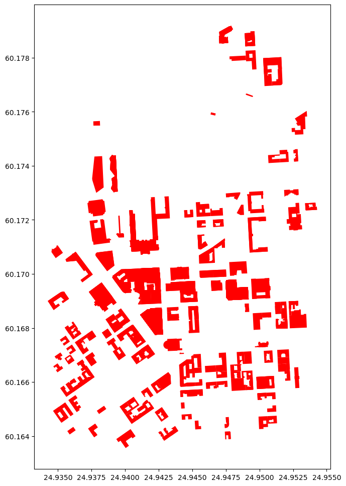
Thus far, we haven’t really made any effort to make our maps visually appealing. Let’s next see how we can adjust the appearance of our map, and how we can visualize many layers on top of each other. Let’s start by visualizing the buildings that we selected earlier and adjust a bit of the colors and figuresize. We can adjust the color of polygons with facecolor parameter and the figure size with figsize parameter that accepts a tuple of width and height as an argument:

ax = join2.plot(facecolor="red", figsize=(12,12))

join2.columns

Index(['geometry', 'addr:city_left', 'addr:country_left',
       'addr:housenumber_left', 'addr:postcode_left', 'addr:street_left',
       'air_conditioning_left', 'brand_left', 'building_left',
       'contact:facebook_left',
       ...
       'building:levels_right', 'architect_right', 'roof:levels_right',
       'seamark:small_craft_facility:category', 'seamark:type',
       'building:part', 'height_right', 'roof:height_right',
       'roof:shape_right', 'indoor'],
      dtype='object', length=385)

Now with the bigger figure size, it is already a bit easier to see the selected buildings that have a restaurant inside them (according OSM). Let’s color our buildings based on the building type. Hence, each building type category will receive a different color:

ax = join2.plot(column="building_left", cmap="RdYlBu", figsize=(12,12), legend=True)

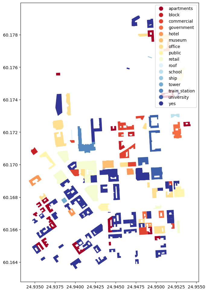
Now we used the parameter column to specify the attribute that is used to specify the color for each building (can be categorical or continuous). We used cmap to specify the colormap for the categories and we added the legend by specifying legend=True.

To get a bit more context to our visualizaton. Let’s also add roads with our buildings. To do that we first need to extract the roads from OSM:

# Get roads (retrieves walkable roads by default)
G = ox.graph_from_polygon(bbox)

# Parse roads from the graph
roads = ox.graph_to_gdfs(G, nodes=False, edges=True) 

Now we can continue and add the roads as a layer to our visualization with gray line color:

# Plot the map again
ax = join2.plot(column="building_left", cmap="RdYlBu", figsize=(12,12), legend=True)

# Plot the roads into the same axis
ax = roads.plot(ax=ax, edgecolor="gray", linewidth=0.75)

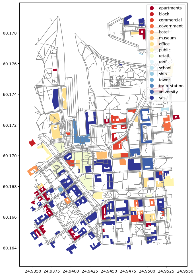
Perfect! Now it is much easier to understand our map because the roads brought much more context (assuming you know Helsinki). We ware able to add the roads to the same map by specifying the ax parameter to point to the axis that we received when first plotting the join2 (i.e. selected buildings). In a similar manner, you can add as many layers in your map as you wish. Let’s still do a small visual trick and specify that the background color in our map is black instead of white. This can be done easily by changing the style of matplotlib visualization renderer:

# Import matplotlib pyplot and use a dark_background theme
import matplotlib.pyplot as plt
plt.style.use("dark_background")

# Plot the map again
ax = join2.plot(column="building_left", cmap="RdYlBu", figsize=(12,12), legend=True)

# Plot the roads into the same axis
ax = roads.plot(ax=ax, edgecolor="gray", linewidth=0.75)

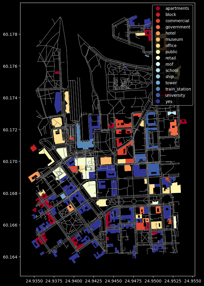
Awesome! Now we have a nice dark theme with our map. With this information you should be able to get going with Exercise 1.

Further information

For further information, we recommend reading the Chapter 6 from the Introduction to Python for Geographic Data Analysis -book.

We also recommend checking the materials from Automating GIS Processes -course (GIS things) and Geo-Python -course (intro to Python and data analysis with pandas). In addition, we always recommend to check the latest documentation from the websites of the libraries:

• geopandas

• osmnx

• matplotlib

• pandas